클라우드 환경에서 머신러닝 서비스 프로토타입 빠르게 만들어보기

Machinelearning
안녕하세요. 머신러닝 엔지니어 김수민입니다. 어반베이스에서 Space의 머신러닝을 이용한 기술 개발을 하고 있습니다.

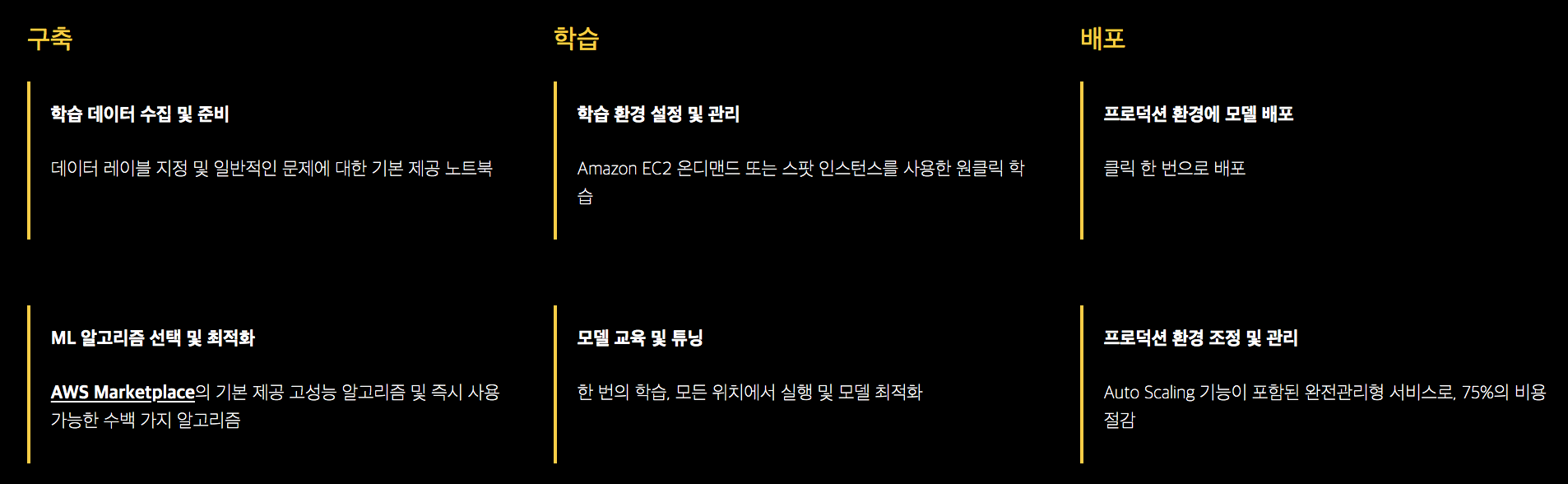
Space는 컴퓨터 비전 영역의 딥러닝을 활용하여 공간을 분류하고, 공간에서 사물을 검출하며 공간의 특성을 분석하는 서비스를 제공합니다. 이것은 AWS의 Sagemaker를 활용하여 학습을 위한 모델 선택부터 배포까지 관리하고 있습니다.

about_sagemaker

*Source: Sagemaker 공식

데이터만 있다면 Sagemaker에서 제공하는 고성능 알고리즘을 사용하여 쉽게 학습해 볼 수 있습니다. 머신러닝 모델의 학습부터 서비스 배포까지 모든 관리 또한 가능하며, AWS의 ML 서비스는 물론 다른 서비스와 통합하여 빠르게 머신러닝 서비스 프로토타입을 만들어 볼 수 있습니다.

Space의 경우 Sagemaker가 제공하는 기본 모델뿐만 아니라 Google의 Tensorflow Object Detection API를 활용하여 정확도를 더욱 높일 수 있는 모델을 검토했습니다. 그 과정에서 시행착오들이 있었는데요. 예를 들면, object detection은 다른 머신러닝 모델 대비 입출력의 데이터 형식이 복잡하다는 특징이 있죠.

이런 시행착오에서 배운 것들을 모아 모델 학습부터 배포까지 빠르게 프로토타입을 만들 수 있는 튜토리얼을 소개해보겠습니다. 그럼 시작 전에 어떤 모델과 데이터를 사용할 지 정리하겠습니다!

Tensorflow Object Detection API

Tensorflow Object Detection API에서 튜토리얼로 제공되는 Oxford-IIIT Pets dataset 과 faster_rnn_resnet_101_coco 모델을 사용합니다.

1) Oxford-IIIT Pets dataset

oxford-pet

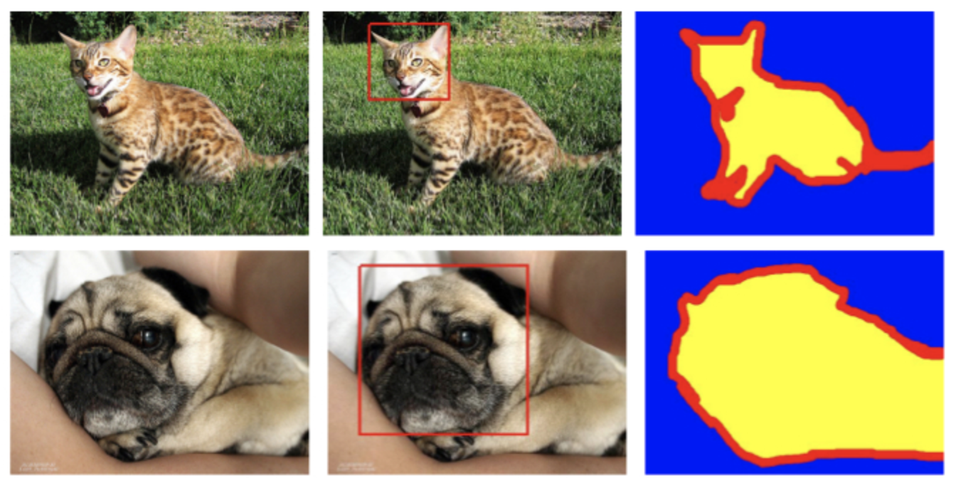
개와 고양이의 품종 별로 클래스 레이블이 있고, 각 이미지 데이터에는 짝으로 개와 고양이의 얼굴 영역과 segmention용 mask 레이블링을 한 데이터가 있습니다.

데이터셋을 다운받으면 images와 annotations 파일이 있는데, images는 이미지 데이터이고 annotations에는 사물 검출 학습에 필요한 검출 상자의 위치, 상자가 가리키는 클래스 정보 등을 담고 있는 xml 파일이 있습니다.

2) Faster R-CNN Resnet-101

object detection에서 two stage 계열의 RCNN 모델 중 속도가 가장 빠른 모델입니다. two stage는 검출 영역을 생성하는 RPN stage와 검출 영역이 정확한 지 판단하는 classifier stage로 나누어져 있습니다. SSD와 YOLO 같은 one stage 계열 모델과 함께 사물 검출 분야에서 많이 사용되고 있는 모델입니다.

Faster R-CNN Resnet-101는 ImageNet 데이터베이스의 이미지를 사전 학습한 Resnet-101를 backbone 네트워크로 사용하는 Faster R-CNN 모델입니다.

다른 모델로 학습하고 싶다면 Object Detection API에서 제공하는 모델 (detection_model_zoo)에서 확인할 수 있습니다.

그럼 시작해볼까요?

Google Colaboratory

그 전에 잠깐, 다른 클라우드 서비스인 colaboratory를 소개하겠습니다.

“Colaboratory는 설치가 필요 없으며 완전히 클라우드에서 실행되는 무료 Jupyter 노트 환경입니다. Colaboratory를 사용하면 브라우저를 통해 무료로 코드를 작성 및 실행하고, 분석을 저장 및 공유하며, 강력한 컴퓨팅 리소스를 이용할 수 있습니다.”

*Source: Colaboratory 공식

왜 Sagemaker가 아닌 다른 서비스를 갑자기 언급했는지 의아하시겠지만, 우리에게 익숙한 jupyter 노트북 환경에 무료로 Tesla K80 GPU를 12시간이나 사용할 수 있다니 안 써 볼 수가 없죠! 12시간보다 긴 학습 시간을 요구하는 모델일 경우에는 충분하지 않겠지만 간단한 학습을 할 때 유용하게 활용할 수 있습니다.

본격적으로 Object Detection API를 사용해봅시다!

1) colab 환경 설정하기

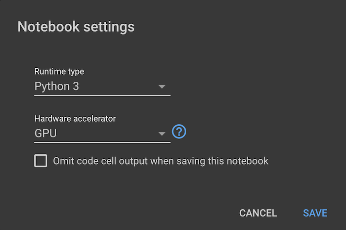
colab notebook을 생성하고 제일 처음으로 할 작업은 GPU 환경으로 설정하기 입니다.

상단 메뉴의 수정 > 노트 설정 을 선택하고 하드웨어 가속기 > GPU 로 변경하면 GPU 환경의 런타임으로 변경됩니다.

gpu_setting

두번째 작업은 파일을 읽고 쓰기 편하게 하기 위해 구글 클라우드의 드라이브를 마운트하는 작업입니다. Mount

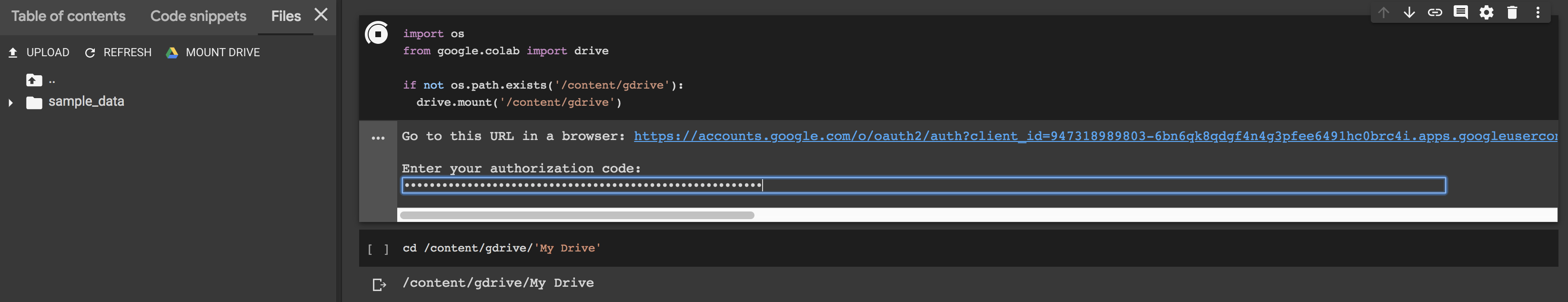
왼쪽 슬라이드바에서 파일 > 드라이브 마운트 (Files > MOUNT DRIVE) 아이콘을 클릭하면 자동으로 코드 스니펫을 생성해줍니다. 셀 실행 시 나오는 링크를 누르고 권한을 허락하면, 드라이브를 마운드하는 키를 발급해줍니다. 이 키를 셀의 출력에 뜬 입력 창에 붙여넣기하면 끝입니다.

import os
from google.colab import drive

if not os.path.exists('/content/gdrive'):
  drive.mount('/content/gdrive')

2) Tensorflow Object Detection API 환경 설정하기

Object Detection API github 레포지토리에는 API를 실행할 때 필요한 환경 설정과 학습, 배포에 관련된 튜토리얼들이 잘 정리되어 있습니다.

설치 튜토리얼을 따라 학습 환경 설정을 colab 환경에서 설정하겠습니다.

먼저 필요한 라이브러리를 설치합니다.

!apt-get install protobuf-compiler python-pil python-lxml python-tk
!pip install Cython
!pip install jupyter
!pip install matplotlib

내 드라이브(My Drive)로 경로를 이동하고 Tensorflow Object Detection API 라이브러리를 다운받습니다.

!cd /content/gdrive/'My Drive'

!git clone https://github.com/tensorflow/models.git

학습 중 모델의 성능 평가를 위해 COCO evaluation metrics api를 설치합니다. 설치 경로를 /content/gdrive/'My Drive'/models/research/로 지정합니다.

!git clone https://github.com/cocodataset/cocoapi.git

!cd cocoapi/PythonAPI; make; cp -r pycocotools /content/gdrive/'My Drive'/models/research/

Tensorflow Object Detection API는 Protobuf를 모델을 설정할 때 사용합니다. Protobufs를 사용할 수 있도록 라이브러리를 컴파일해줍니다.
컴파일할 경로인 /content/gdrive/'My Drive'/models/research/로 이동합니다.

!cd /content/gdrive/'My Drive'/models/research

!protoc object_detection/protos/*.proto --python_out=.

Object Detection API의 라이브러리를 setup.py 파일로 설치합니다. 설치할 setup.py 파일이 두 가지가 있는데, 첫번째는 /content/gdrive/'My Drive'/models/research에 있는 파일, 두번째는 /content/gdrive/'My Drive'/models/research/slim에 있는 파일입니다.

!python setup.py build
!python setup.py install

slim 폴더에 있는 setup.py를 설치합니다.

!cd /content/gdrive/'My Drive'/models/research/slim

!python setup.py build
!python setup.py install

라이브러리를 PYTHONPATH에 추가합니다. 이 작업은 /content/gdrive/'My Drive'/models/research/에서 합니다.

!cd /content/gdrive/'My Drive'/models/research

%set_env PYTHONPATH=/content/gdrive/'My Drive'/models/research:/content/gdrive/'My Drive'/models/research/slim

마지막으로 Tensorflow Object Detection API의 설치가 제대로 되었는지 확인합니다.

!python object_detection/builders/model_builder_test.py

짝짝짝! 마지막 줄에 OK가 출력되었다면 성공적으로 설치를 마쳤습니다!

3) Oxford-IIIT Pets dataset 다운 후 tfrecord 형식으로 빌드하기

데이터셋을 다운받고 각각 images 폴더와 annotations 폴더에 압축을 풉니다.

!wget http://www.robots.ox.ac.uk/~vgg/data/pets/data/images.tar.gz
!wget http://www.robots.ox.ac.uk/~vgg/data/pets/data/annotations.tar.gz
!tar -xvf images.tar.gz
!tar -xvf annotations.tar.gz

pbtxt

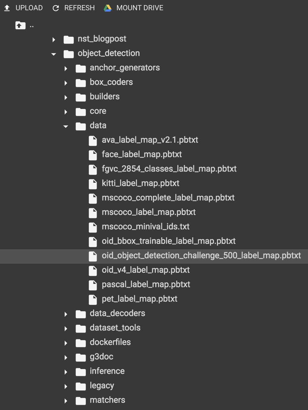
tfrecord 형식으로 빌드할 때 데이터셋의 레이블을 명시한 label map 파일이 필요합니다. 튜토리얼용 pet_label_map.pbtxt는 이미 object_detection/data/에 준비되어 있지만, 커스텀 데이터셋으로 학습을 하는 경우에는 Object Detection API의 pbtxt 파일 형식에 맞추어 준비합니다. 그리고 나머지 데이터의 위치(--data_dir)와 빌드된 tfrecord 파일이 저장될 위치(--output_dir)를 지정해주고 명령을 실행합니다.

!python object_detection/dataset_tools/create_pet_tf_record.py \
  --label_map_path=object_detection/data/pet_label_map.pbtxt \
  --data_dir=/content/gdrive/'My Drive'/models/research \
  --output_dir=/content/gdrive/'My Drive'/models/research

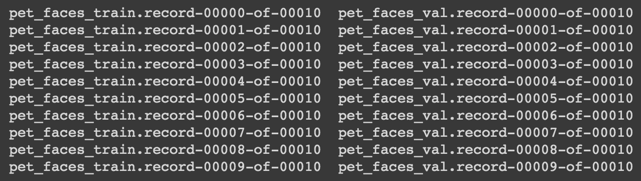
다음 명령어로 생성된 tfrecord 파일을 확인할 수 있습니다.

ls *.record*

tfrecord_results

4) Pre-trained된 모델 다운받기

coco 데이터셋으로 미리 학습된 모델을 사용하여 전이학습(trasfer learning)을 합니다. 새로운 모델로 학습할 때보다 이미지에 대한 분포를 더 많이 학습했기 때문에 효율적으로 학습할 수 있는 장점이 있습니다. Object Detection API의 detection model zoo 페이지 COCO-trained-models 항목에서 모델을 다운받거나 링크를 복사해서 드라이브에 바로 다운받을 수 있습니다.

coco-trained-model

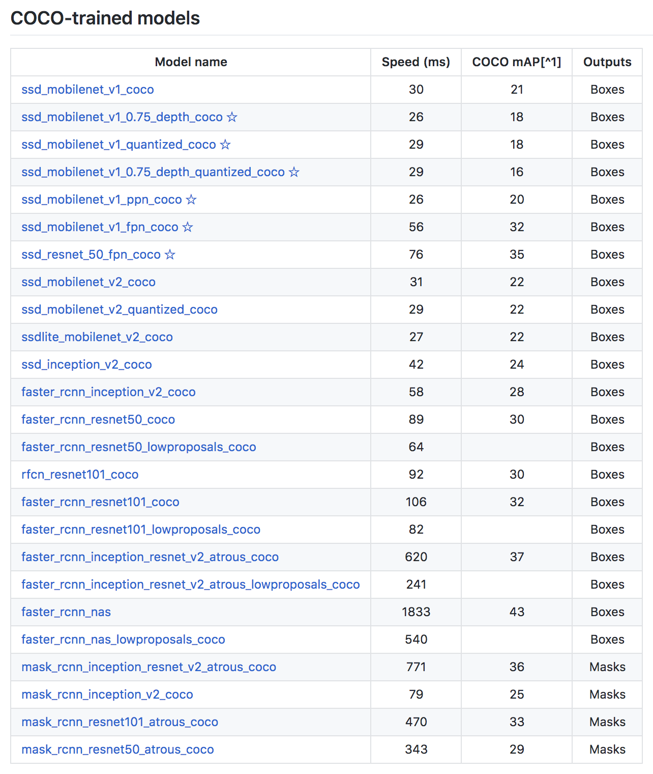
필요한 모델인 faster_rcnn_resnet101_coco을 다운받습니다.

!wget http://download.tensorflow.org/models/object_detection/faster_rcnn_resnet101_coco_2018_01_28.tar.gz
!tar -xvf faster_rcnn_resnet101_coco_2018_01_28.tar.gz
!cp faster_rcnn_resnet101_coco_2018_01_28/model.ckpt.* .

5) config 파일 수정하기

Tensorflow Object Detection API는 모델의 구조나 학습을 위한 파라미터, 파이프라인을 모두 .config 파일로 관리합니다. 튜토리얼을 위한 템플릿 config 파일은 object_detection/samples/configs 폴더에 있습니다.

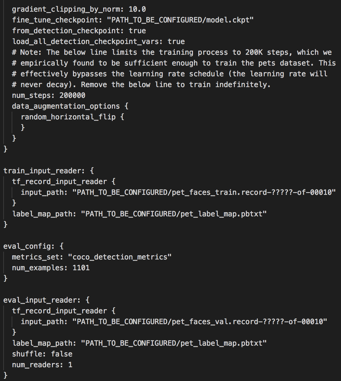
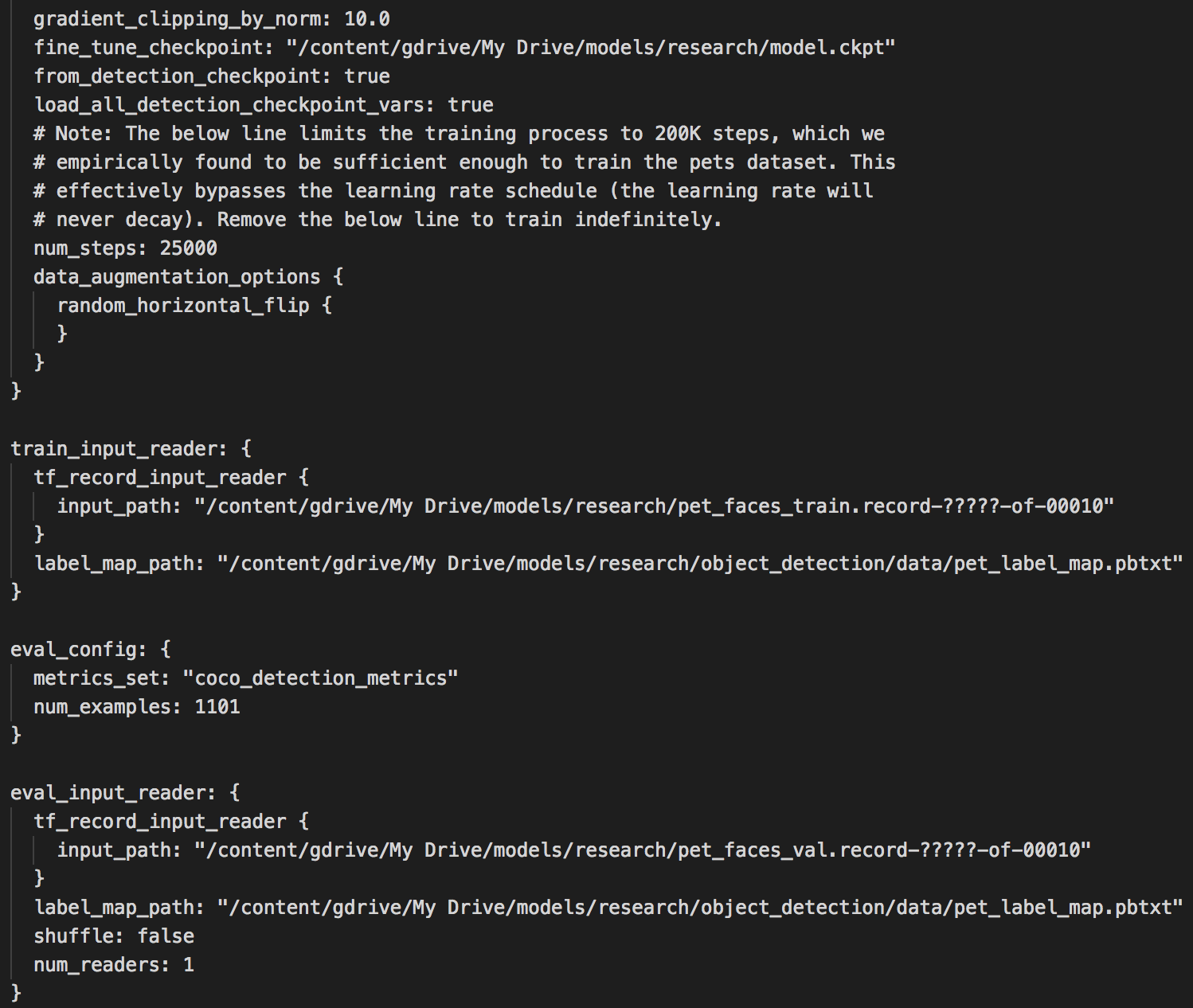
faster-coco-pet-config pet-config-modified

파라미터들은 기본값을 쓰겠지만 12시간 안에 학습하도록 num_steps를 25000으로 바꾸겠습니다. Oxford-IIIT Pets dataset에는 총 7349개의 이미지가 있고, train dataset으로 70%를 사용합니다. 한 스탭에 사용하는 데이터 양을 뜻하는 batch_size가 1이기 때문에 지정한 25000번 동안 train dataset을 약 4번 반복(4 epoch)하면서 학습합니다.

그리고 PATH_TO_BE_CONFIGURED 부분을 각 파일이 위치한 경로로 수정해야 합니다.

fine_tune_checkpoint 경로는 4)에서 다운받은 model.ckpt.* 가 저장되어 있는 경로인 /content/gdrive/My Drive/models/research/model.ckpt로 수정합니다.
각 train과 evaluation tfrecord의 경로는 /content/gdrive/My Drive/models/research 로 수정합니다. record의 이름도 동일한지 확인합니다.(pet_faces_train/pet_faces_val)
pet_label_map.pbtxt 파일의 경로도 /content/gdrive/My Drive/models/research/object_detection/data/ 로 수정합니다.

이 작업을 직접 드라이브에서 다운받고 수정 후 재업로드해도 되고, 코드로도 할 수 있습니다.

!cp object_detection/samples/configs/faster_rcnn_resnet101_pets.config .

!sed -i “s|PATH_TO_BE_CONFIGURED|/content/models/research|g” faster_rcnn_resnet101_pets.config

!sed -i “s|/content/models/research/pet_label_map.pbtxt|/content/models/research/object_detection/data/pet_label_map.pbtxt|g” faster_rcnn_resnet101_pets.config

6) 학습하기

여기까지 잘 하셨습니다! 그럼 뚜둔 드디어 학습을 해보겠습니다.

PIPELINE_CONFIG_PATH: faster_rcnn_resnet101_pets.config 파일이 있는 경로를 기입합니다.
MODEL_DIR: 학습 도중 event와 checkpoint 파일을 저장할 위치를 지정합니다.

\# From the tensorflow/models/research/ directory

PIPELINE_CONFIG_PATH='/content/gdrive/"My Drive"/models/research/faster_rcnn_resnet101_pets.config'
MODEL_DIR='/content/gdrive/"My Drive"/models/research/model_ckpt'
SAMPLE_1_OF_N_EVAL_EXAMPLES=1

!python object_detection/model_main.py \
  --pipeline_config_path={PIPELINE_CONFIG_PATH} \
  --model_dir={MODEL_DIR} \
  --sample_1_of_n_eval_examples=$SAMPLE_1_OF_N_EVAL_EXAMPLES \
  --alsologtostderr

Created TensorFlow device (/job:localhost/replica:0/task:0/device:GPU:0 with 10805 MB memory) -> physical GPU (device: 0, name: Tesla K80, pci bus id: 0000:00:04.0, compute capability: 3.7) 가 출력되었다면 GPU 환경에서 학습이 진행됩니다.

그럼 학습이 끝날 때까지 기다립니다…

later_pic

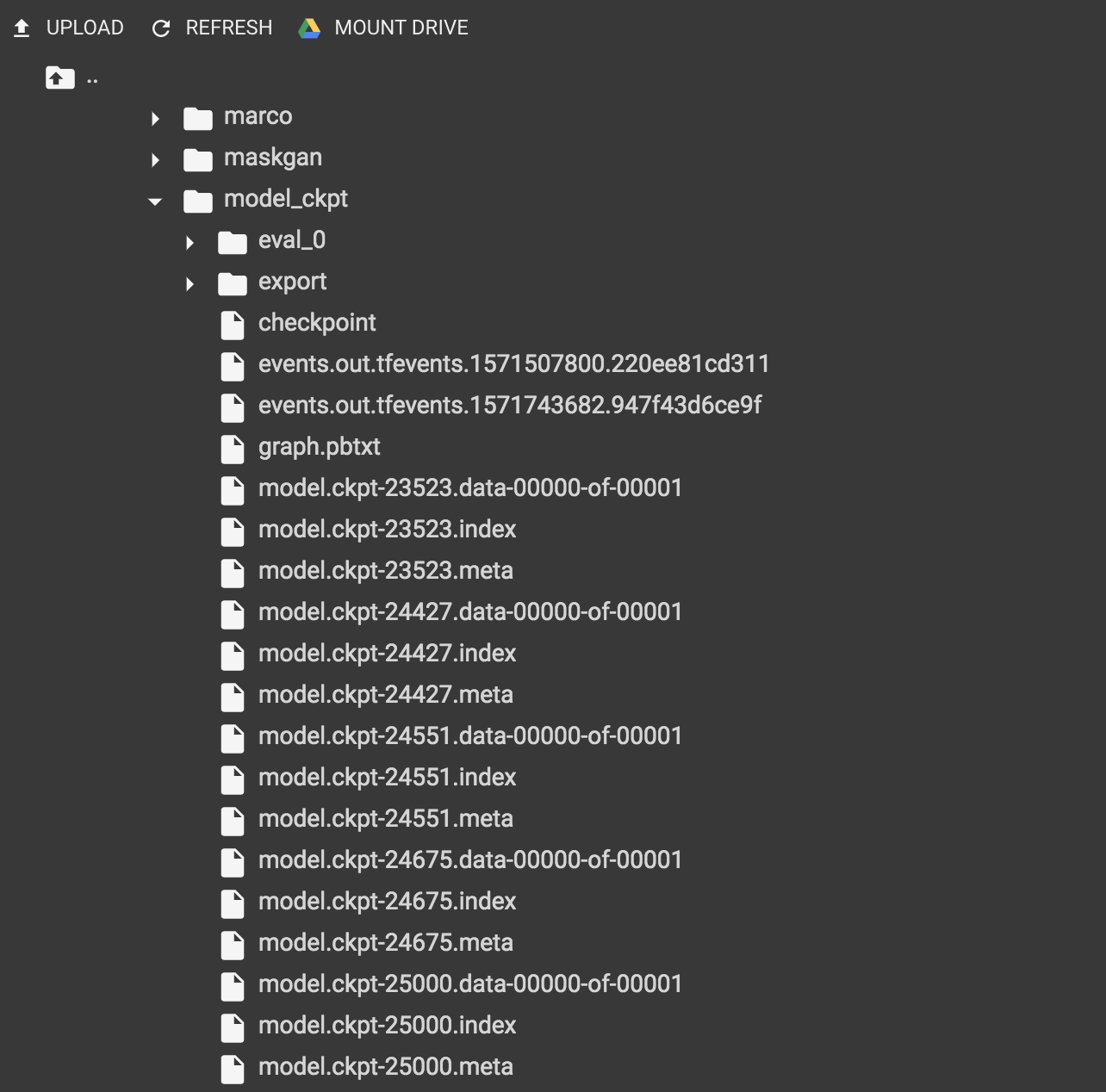
…학습이 잘 끝났나요?
학습이 잘 되었다면 model_dir 인자로 지정한 경로에 checkpoint가 저장되어 있습니다.

model_ckpt

성능 평가는 다음과 같습니다. metric

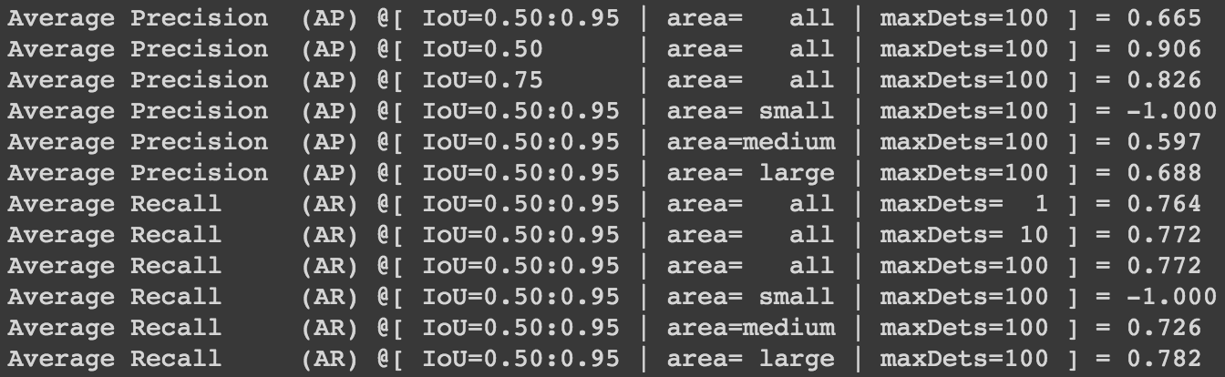
위 성능 결과는 COCO evaluation metrics를 사용합니다. 평가에 대한 정보는 여기를 참고해 주세요. 이 튜토리얼에서는 생략했지만 colab에서 tensorboard를 통해서 학습이 어떻게 진행됐는지 확인이 가능하니 참고 바랍니다.

그럼 이제 배포를 하고 결과값을 확인해볼까요? 배포에는 Tensorflow Serving을 사용합니다.

Tensorflow Serving

“제품 환경을 위해 디자인 되었으며, 머신러닝 모델을 위해 유연하며 고성능의 서빙 시스템을 제공합니다. 텐서플로우 서빙을 통해 같은 서버 아키텍쳐와 API를 유지하는 동안, 새로운 알고리즘과 실험을 쉽게 배포할 수 있습니다.”

*Source:Tensorflow Serving 공식

Tensorflow Serving은 Docker 기반으로 여러 플랫폼에서 유연하게 구축이 가능한 장점이 있습니다. AWS에서도 Tensorflow 모델에 대한 배포 이미지로 Tensorflow Serving을 사용할 수 있도록 지원합니다.

Tensorflow Serving 구조

tf-serving-structure

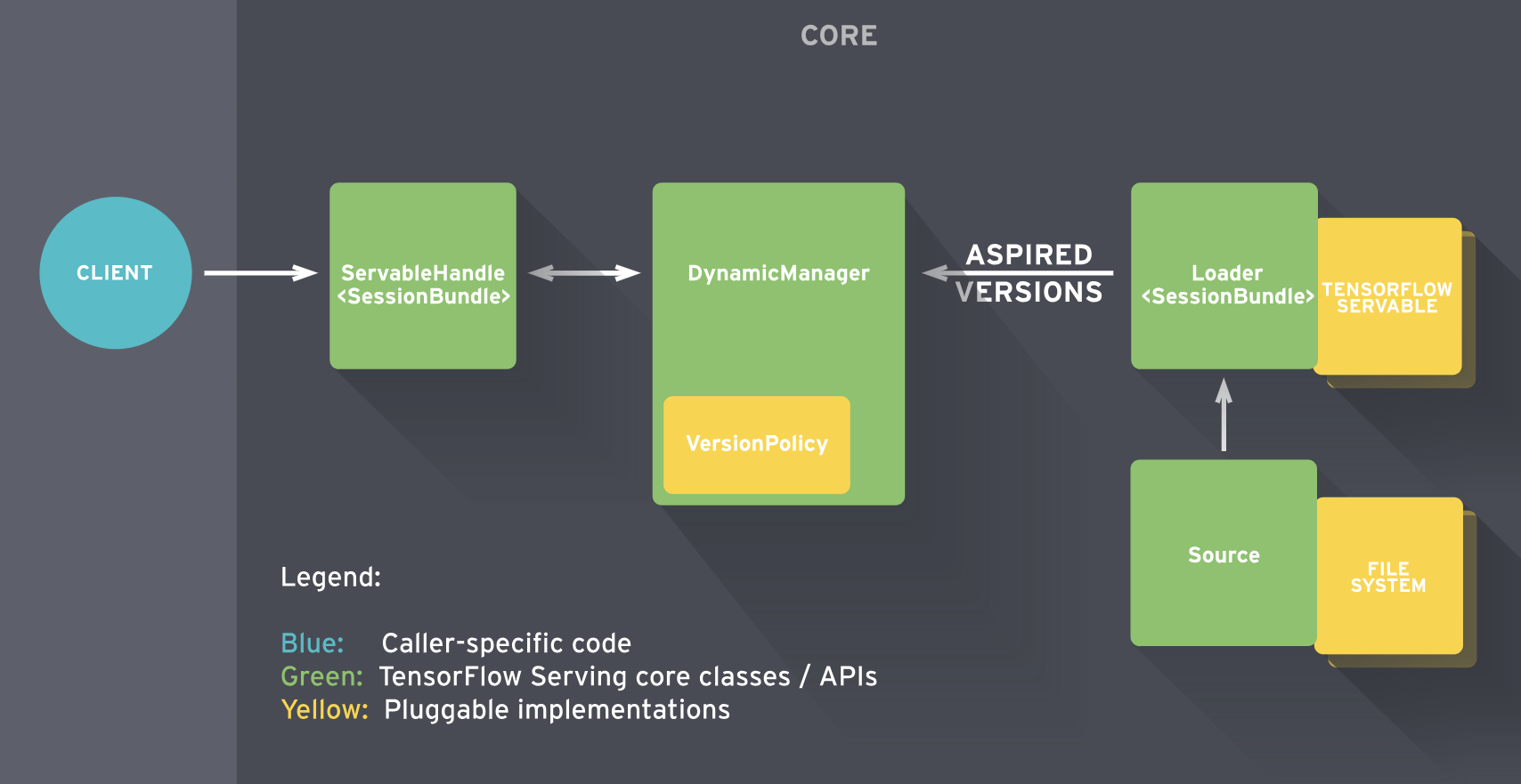
Servables
- 클라이언트가 계산을 수행하는데 사용하는 기본 object(perform computation)
- model 저장
- 4개의 component의 중심
Loaders
- servable(model)의 life cycle 관리
- manager를 위한 임시 저장소(temporary storage for the manager)
Sources
- contain servables
- gateway
- loader로 올림
- 모델의 다른 버전 track
Managers
- full lifecycle 관리

*Source: https://zzsza.github.io/data/2018/07/12/tensorflow-serving-tutorial

그럼 colab 환경에서 학습이 완료된 모델을 이어서 배포까지 해보겠습니다.

Colab 환경에서 Tensorflow Serving 테스트 해보기

1) 수정된 `exporter.py` 만들기

Tensorflow Serving은 SavedModel 포맷*의 saved_model.pb와 모델을 복구하기 위한 체크포인트 정보가 담긴 variable 파일이 필요합니다. Tensorflow Object Detection API의 exporter.py로 SavedModel을 추출할 때 그 기능이 없기 때문에 코드의 수정이 필요합니다.

(* 참고 SavedModel은 변수값과 상수를 포함하고 직렬화된 시그니처와 이를 실행하는 데 필요한 상태를 담은 디렉토리입니다.)

코드를 수정한 참고 github의 코드를 exporter_savedmodel.py로 저장하고 다음과 같이 수정합니다.

> Line 72: change optimize_tensor_layout=True ==>  layout_optimizer=True
>
> Line 327-329:<p>
> preprocessed_inputs, true_image_shapes = detection_model.preprocess(inputs)<p>
> output_tensors = detection_model.predict(preprocessed_inputs, true_image_shapes)<p>
> postprocessed_tensors = detection_model.postprocess(output_tensors, true_image_shapes)

Object Detection API가 저장되어 있는 /content/gdrive/My Drive/models/research/object detection 에 파일을 업로드합니다.

2) SavedModel 포맷 만들기

import tensorflow as tf

from object_detection.utils.config_util import create_pipeline_proto_from_configs
from object_detection.utils.config_util import get_configs_from_pipeline_file
import object_detection.exporter_savedmodel

# export하는 학습 모델의 Configuration 파일 경로
config_pathname = '/content/gdrive/My Drive/models/research/faster_rcnn_resnet101_pets.config'

# export하는 학습 모델의 checkpoint 경로
trained_model_dir = '/content/gdrive/My Drive/models/research/model_ckpt' 

# Configuration 파일에서 proto를 생성
configs = get_configs_from_pipeline_file(config_pathname)
pipeline_proto = create_pipeline_proto_from_configs(configs=configs)

# model checkpoint 경로에서 .ckpt와 .meta 파일을 읽기
checkpoint = tf.train.get_checkpoint_state(trained_model_dir)
input_checkpoint = checkpoint.model_checkpoint_path

# 모델 버전
model_version_id = 1

# Output 디렉토리 경로
output_directory = '/content/gdrive/My Drive/models/research/pet_saved_model' + '/' + str(model_version_id)

# 모델 export 하기
object_detection.exporter_savedmodel.export_inference_graph(input_type='encoded_image_string_tensor', pipeline_config=pipeline_proto, trained_checkpoint_prefix=input_checkpoint, output_directory=output_directory)

exporter는 세 가지 input 방식을 지정할 수 있습니다. export_inference_graph의 input_type 인자를

input_type='image_tensor'로 하면 image tensor를 json serializion 합니다.
input_type='encoded_image_string_tensor'로 하면 base64를 json serializion 합니다.
input_type='tf_example'로 하면 tf example를 json serializtion 합니다.

이번에는 두 번째 방법으로 export 했습니다.

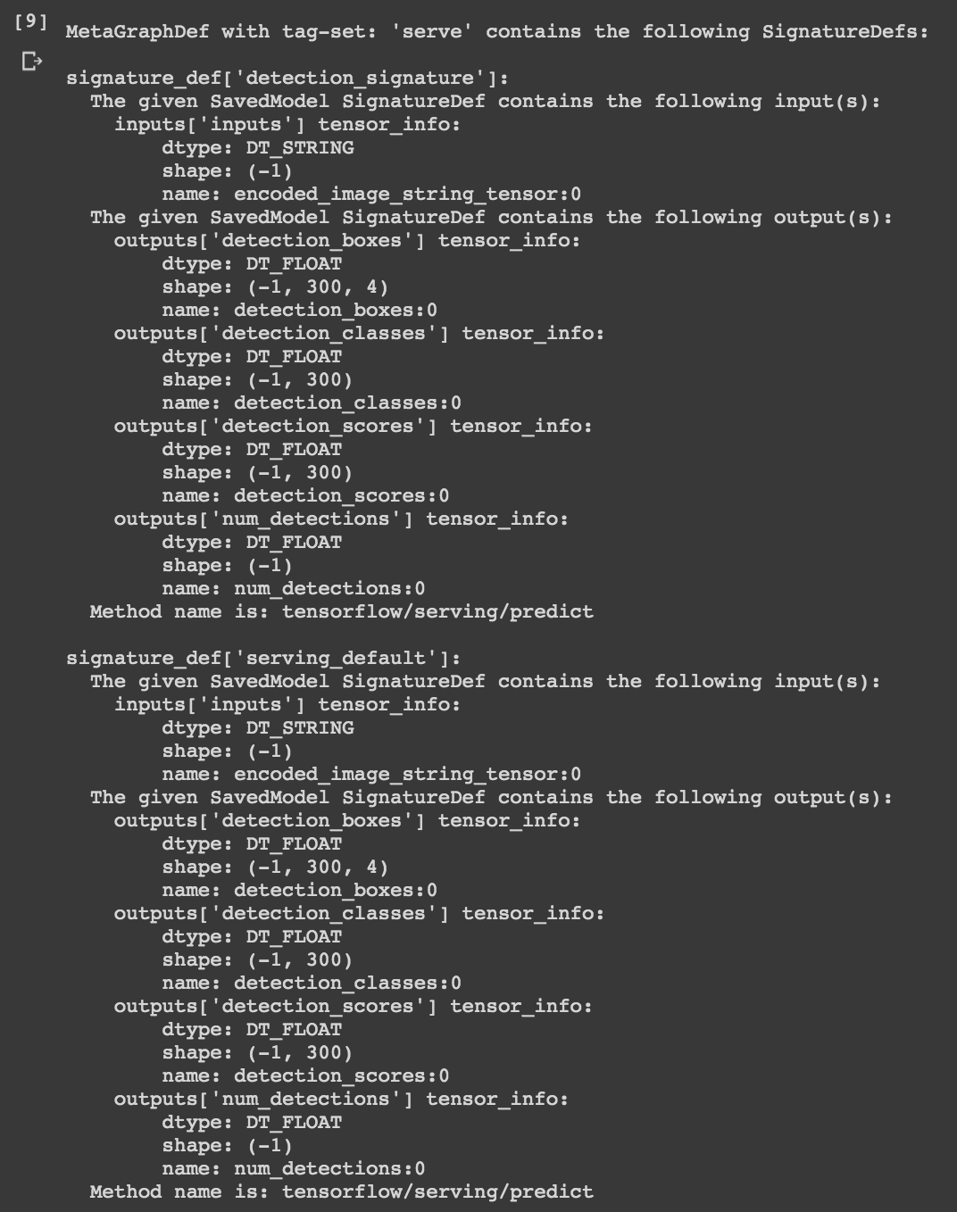
export된 saved_model에 대한 정보를 볼 수 있습니다.

!saved_model_cli show --dir '/content/gdrive/My Drive/models/research/pet_saved_model/1' --all

exported_model

3) Tensorflow Serving 다운받고 설치하기

!echo "deb http://storage.googleapis.com/tensorflow-serving-apt stable tensorflow-model-server tensorflow-model-server-universal" | tee /etc/apt/sources.list.d/tensorflow-serving.list && \
curl https://storage.googleapis.com/tensorflow-serving-apt/tensorflow-serving.release.pub.gpg | apt-key add -

!apt update

!apt-get install tensorflow-model-server

4) Tensorflow Serving 실행하기

Tensorflow Serving을 시작하고 모델을 로드합니다. Tensorflow Serving은 gRPC와 REST API 두가지 방식으로 처리할 수 있습니다. 이번에는 REST API 방식으로 합니다.

rest_api_port: REST 요청을 받을 포트 번호를 씁니다. gRPC는 8500, REST는 8501을 주로 사용합니다.
model_name: REST 요청의 URL에 사용할 이름을 지정합니다.
model_base_path: 로드할 모델을 저장한 경로를 지정합니다.

os.environ["MODEL_DIR"] = '/content/gdrive/My Drive/models/research/pet_saved_model'

%%bash --bg 
nohup tensorflow_model_server \
  --rest_api_port=0.0.0.0:8501 \
  --model_name=fashion_model \
  --model_base_path='/content/gdrive/My Drive/models/research/pet_saved_model' >server.log 2>&1

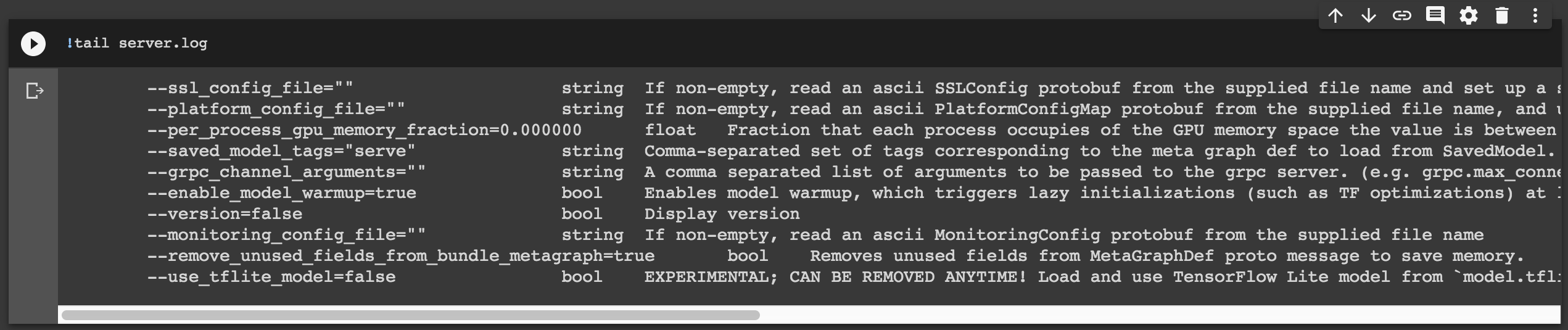
!tail server.log

다음과 같은 결과가 나오면 잘 구동이 된 것입니다. server_log

5) Tensorflow Serving에 추론 요청 보내기

요청을 보내기 위한 이미지를 구글에서 가져옵니다.

test image

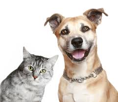
그런 다음 학습한 모델이 잘 추론하는지 확인해보겠습니다.

!pip install -q requests

추론할 이미지를 base64로 변환 후 Tensorflow Serving 호출 방식인 json에 serialize 합니다.

import json
import base64
import request

filepath = '/content/gdrive/My Drive/models/research/object_detection/test_images/<TEST_IMAGE>.jpeg'

with open(filepath, "rb") as image:
  image_data = image.read()
  encoded_input_string = base64.b64encode(image_data).decode('utf-8')

data = json.dumps({"signature_name": "serving_default", "instances": [{"inputs": {'b64': encoded_input_string}}]})

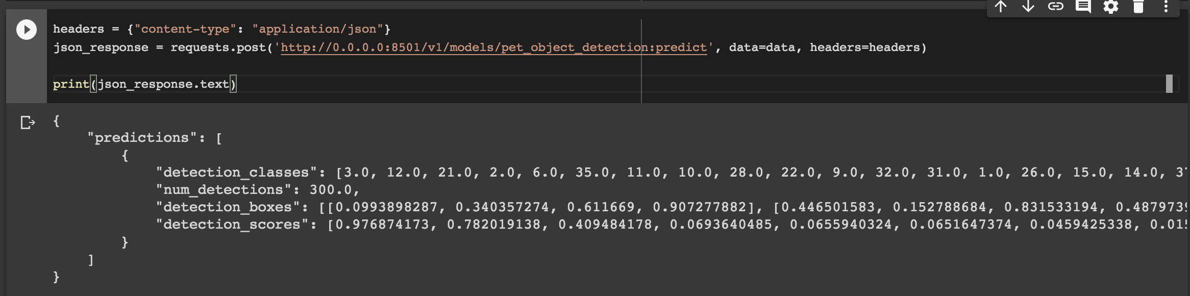
이제 Tensorflow Serving에 추론 요청을 보내겠습니다.

headers = {"content-type": "application/json"}
json_response = requests.post('http://0.0.0.0:8501/v1/models/pet_object_detection:predict', data=data, headers=headers)

print(json_response.text)

다음과 같이 추론 결과가 반환됩니다!

serving_result

Object Detection API의 튜토리얼에 있는 시각화 코드로 검출 결과를 시각화 할 수 있습니다.

여기서는 결과 이미지만 보겠습니다. 나머지 자세한 코드는 아래에 링크된 colab notebook을 확인해주세요.

inference_result

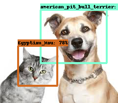
오! 높은 확률로 잘 검출한 것 같습니다! 이미지에는 안 보이지만 추론 결과를 보면 american_pitbull_terrior는 97% 의 확률이네요.

이렇게 학습, 배포, 추론을 colab 환경에서 해보았습니다!

Sagemaker에서 배포하기

이제 테스트를 끝내고 서비스할 수 있도록 Sagemaker에 endpoint를 생성하겠습니다.

1) Docker 설치

“Docker는 애플리케이션을 신속하게 구축, 테스트 및 배포할 수 있는 소프트웨어 플랫폼입니다. Docker는 소프트웨어를 컨테이너라는 표준화된 유닛으로 패키징하며, 이 컨테이너에는 라이브러리, 시스템 도구, 코드, 런타임 등 소프트웨어를 실행하는 데 필요한 모든 것이 포함되어 있습니다. Docker를 사용하면 환경에 구애받지 않고 애플리케이션을 신속하게 배포 및 확장할 수 있으며 코드가 문제없이 실행될 것임을 확신할 수 있습니다.”

*Source: AWS 공식, Docker란 무엇입니까?

도커는 Tensorflow Serving울 구동하는 가상 환경 이미지를 생성하고, Sagemaker는 EC2 인스턴스에서 배포 이미지를 서비스하는 방식으로 endpoint를 생성합니다. 다음 링크를 참고하여 로컬 운영체제에 맞게 도커를 설치해주세요.

2) dockerfile 구성하기

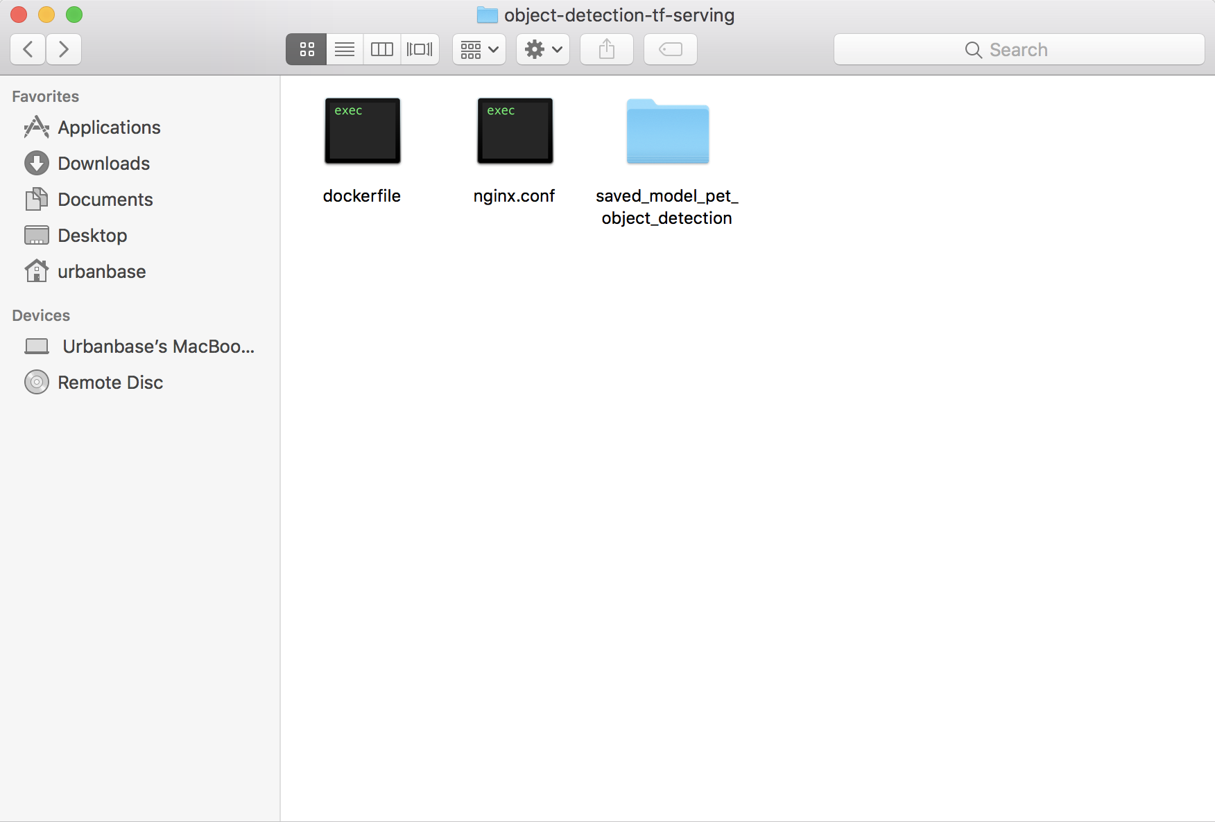
Sagemaker가 Docker image를 실행하고 Tensorflow Serving을 구동할 수 있도록 필요한 파일을 구성합니다. 이 과정은 local에 임의의 폴더(여기서는 object-detection-tf-serving)를 만들어서 진행합니다.

dockerfile: docker image를 빌드할 때 패키지나 데이터를 추가하기 위한 명령어를 나열한 파일입니다.
nginx.conf: Sagemaker endpoint에 요청된 것을 docker image 상에서 구동된 Tensorflow Serving으로 보내는 역할을 합니다.
saved_model_pet_object_detection: Tensorflow Serving에 로드할 모델을 준비합니다.

docker_setting

Dockerfile

# 공식 tensorflow serving image 를 사용하기 위해 base image로 설치합니다.
FROM tensorflow/serving:latest-gpu

# Sagemaker에서 TF Serving으로 추론을 리버스 프록시하는 역할인 NGINX를 설치합니다.
RUN apt-get update 
RUN apt-get install -y --no-install-recommends nginx git

# 모델 폴더를 컨테이너로 복사합니다.
COPY saved_model_pet_object_detection /saved_model_pet_object_detection

# NGINX 설정 파일을 컨테이너로 복사합니다.
COPY nginx.conf /etc/nginx/nginx.conf

#  NGNIX와 TF Serving을 실행하고 모델을 바라보도록 합니다.
ENTRYPOINT service nginx start | tensorflow_model_server --rest_api_port=8501 \
 --model_name=pet_object_detection \
 --model_base_path=/saved_model_pet_object_detection

Nginx.conf

events {
    # determines how many requests can simultaneously be served
    # https://www.digitalocean.com/community/tutorials/how-to-optimize-nginx-configuration
    # for more information
    worker_connections 2048;
}

http {
  server {
    # 서버가 포트 8080를 확인하도록 합니다.
    listen 8080 deferred;
    
    client_max_body_size 5m;

    # Sagemaker에서 TF Serving으로 리다이렉트 합니다.
    location /invocations {
      proxy_pass http://localhost:8501/v1/models/pet_object_detection:predict;
    }

    # Sagemaker의 상태 확인을 합니다.
    location /ping {
      return 200 "OK";
    }
  }
}

saved_model_pet_object_detection 폴더 구성

saved_model_pet_object_detection
├── 1
|   ├── variables
|   |   ├── variables.data-00000-of-00001
|   |   ├── variables.index
|   └── saved_model.pb

3) AWS Credentials

AWS CLI를 활용해 local ECR로 Docker image를 업로드하기 위해서 지격 증명 파일의 정보를 구성합니다. 다음의 AWS CLI 구성을 참고합니다.

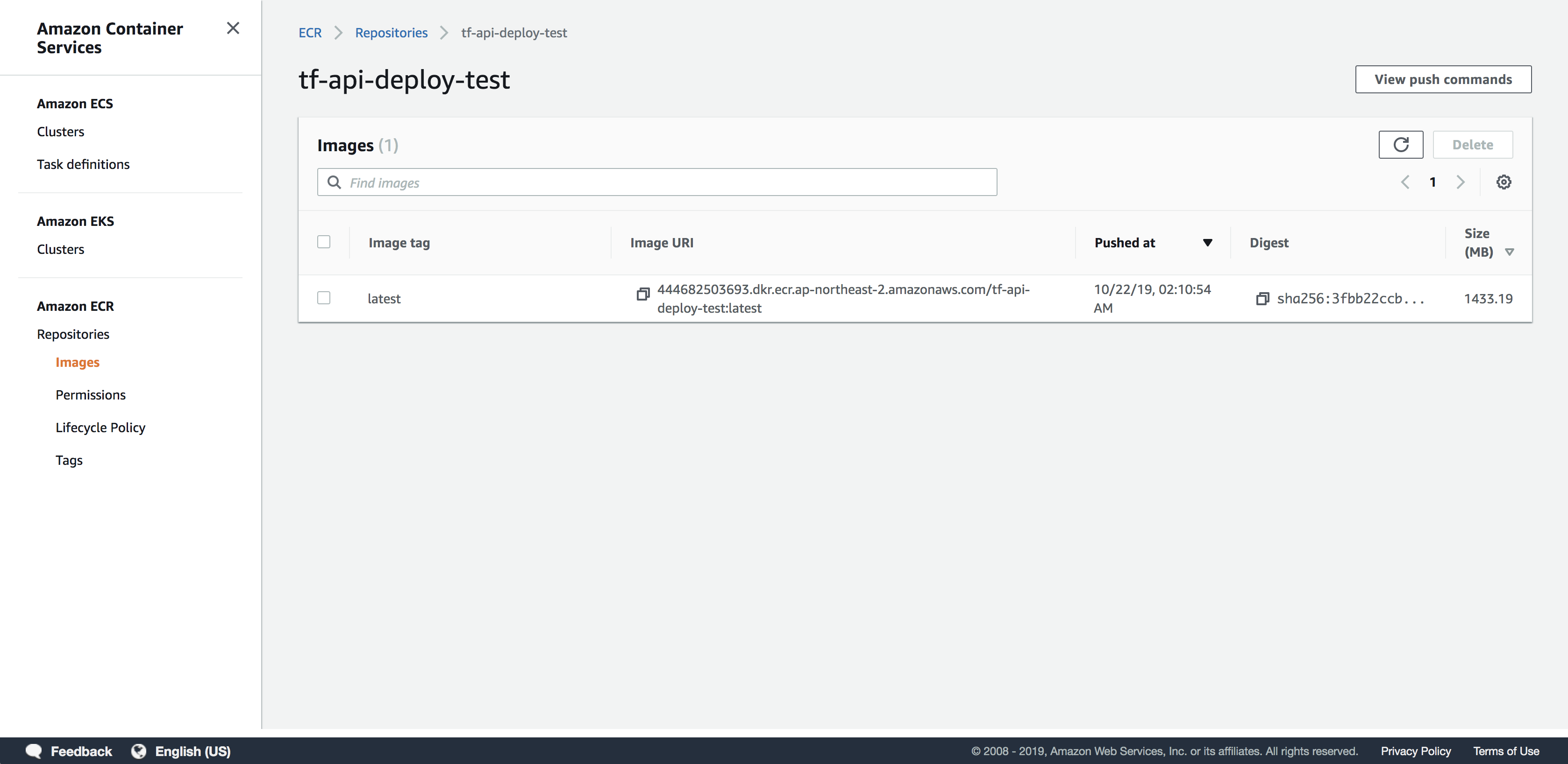
4) ECR 업로드

AWS ECR(Amazon EC2 Container Registry)에 Docker Image를 업로드합니다. 먼저 ECR에 레포지토리를 만들고 제공되는 업로드의 각 과정을 복사&붙여넣기 하면 쉽게 진행할 수 있습니다.

ecr-aws-cli

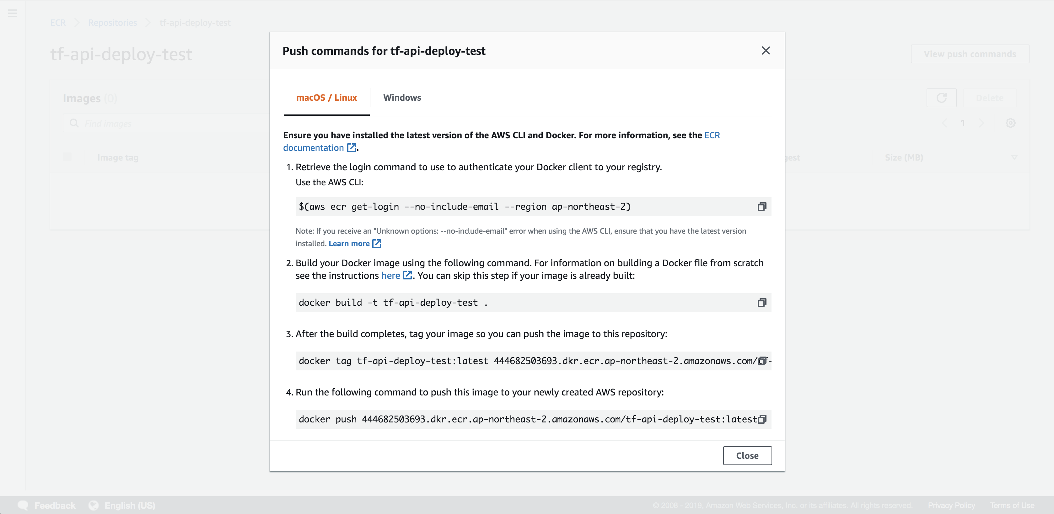
업로드 되었습니다!

ecr-uploaded

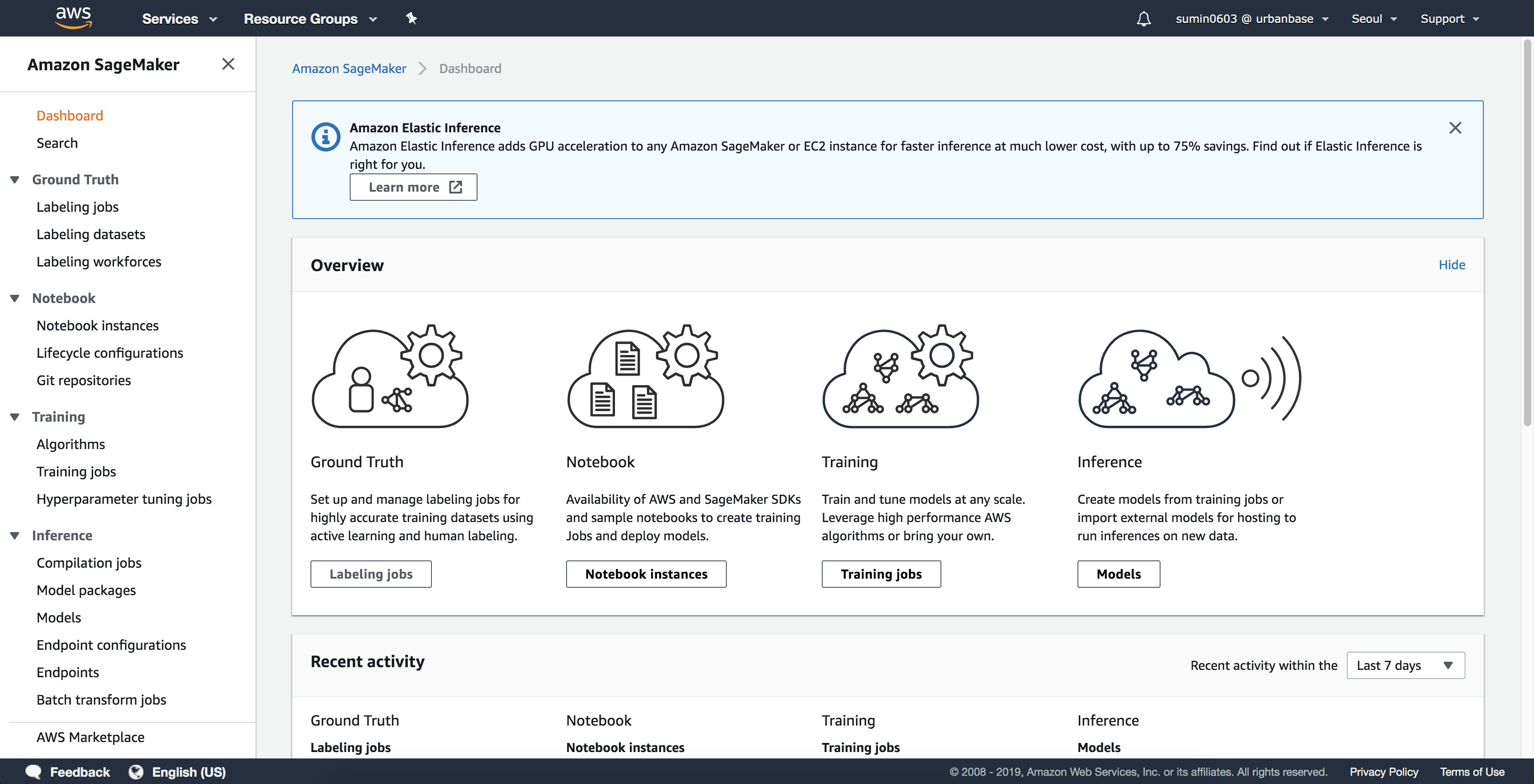
5) Sagemaker에서 엔드포인트 만들기

업로드가 완료된 ECR에서 Image URI를 복사한 후 Sagamaker 서비스에서 endpoint를 생성해보도록 하겠습니다. endpoint가 생성이 되면 과금이 발생합니다. 테스트가 끝나면 꼭 삭제합니다.

sagemaker_main

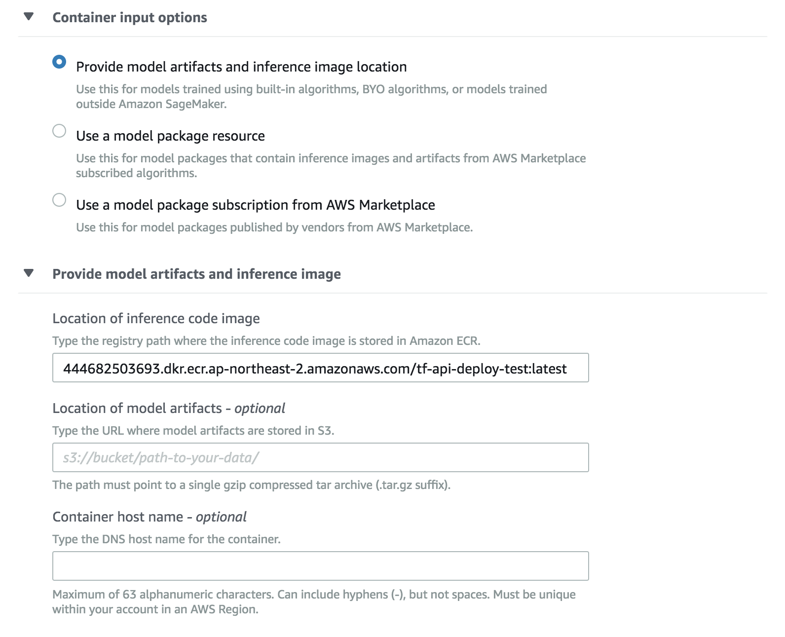
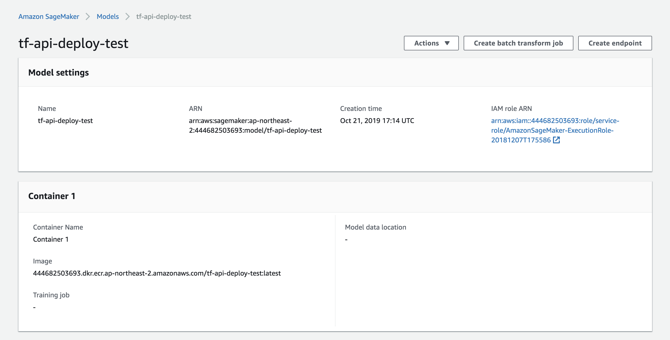
a. Sagemaker의 메뉴 창, 추론(Inference) 메뉴의 모델(Models)에서 모델 생성(Create Model)을 합니다. Container definition 1에서 ECR에서 생성한 이미지 URL을 적용합니다.

create_model model-container

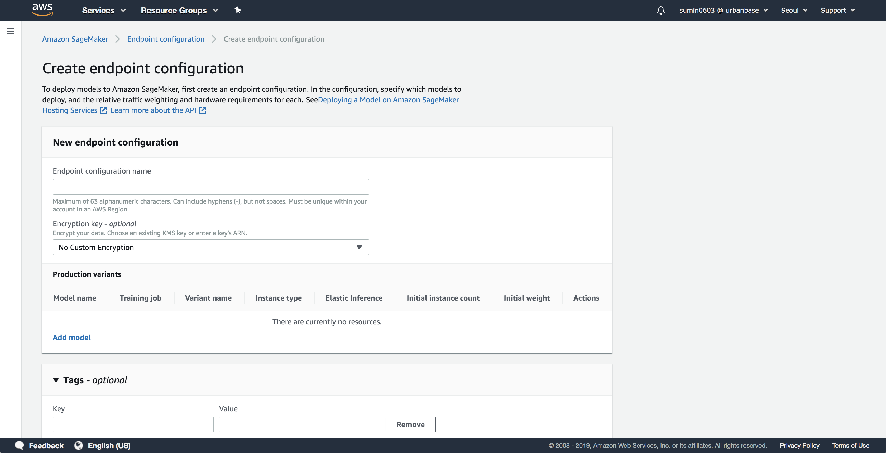
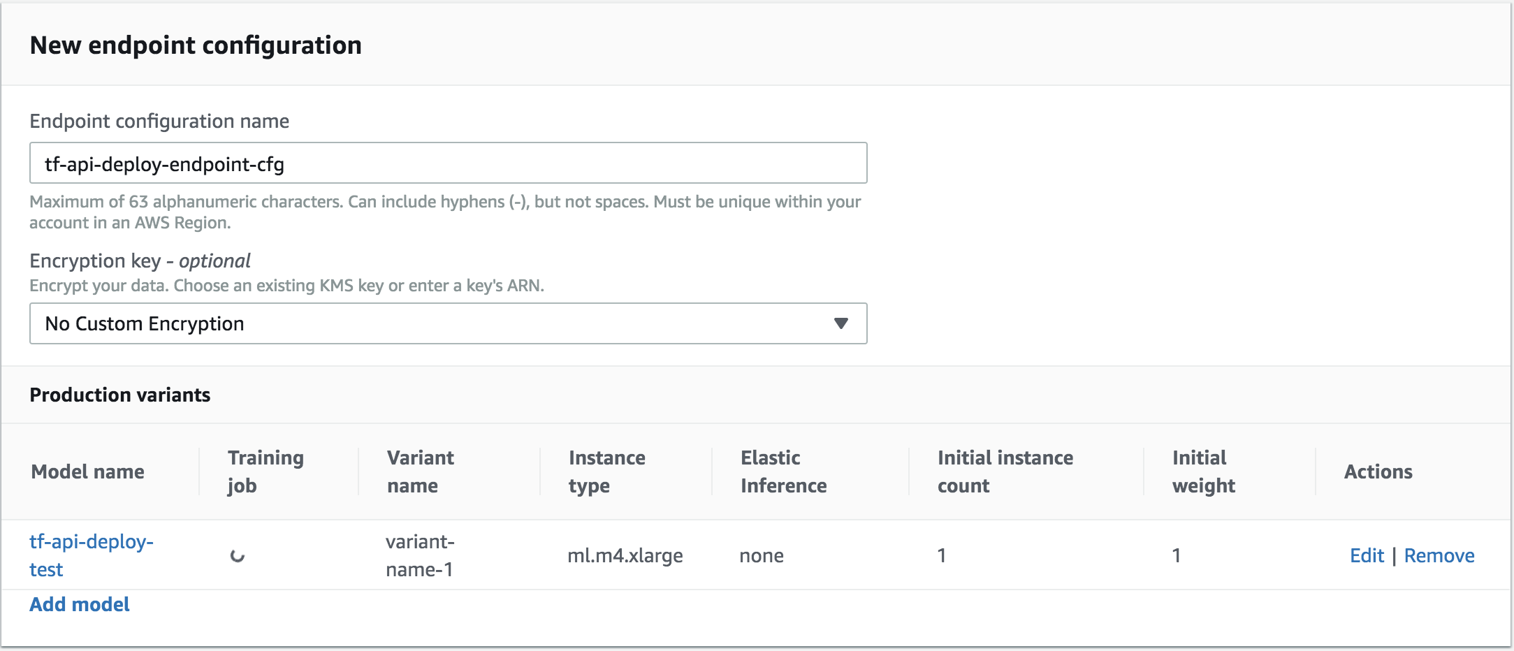
b. 엔트포인트 구성 메뉴에서 엔트포인트 구성(Create endpoint configuration)을 합니다. Endpoint configuration name에 구성 이름을 정하고 Add model에서 모델 컨테이너를 연결합니다. Actions의 Edit에서 Instance type, Elastic Inference를 지정할 수 있습니다.

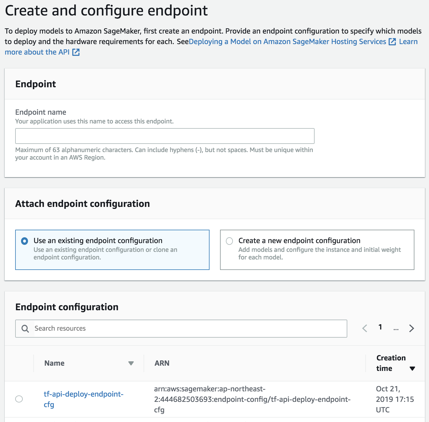
endpoint_configure edit_production_variants

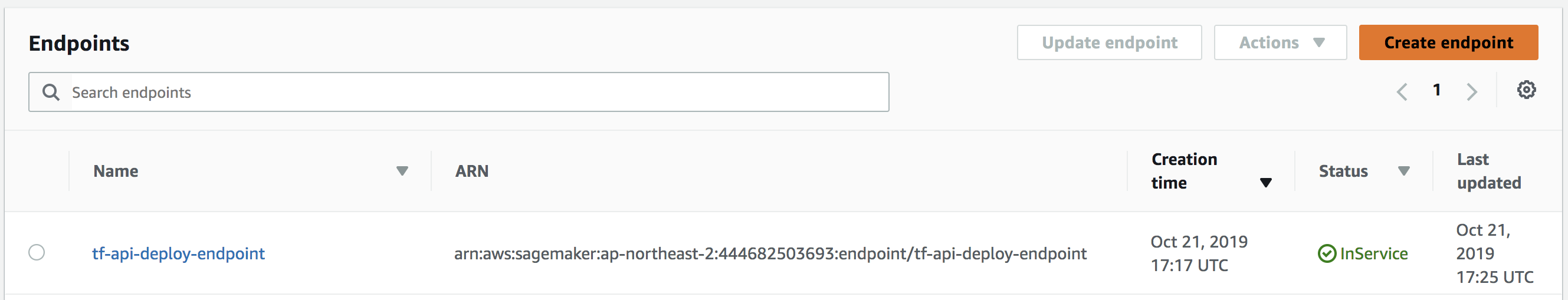
c. 엔트포인트를 생성합니다. Endpoint name으로 이름을 지정하고, Endpoint configuration에서 앞에서 생성한 엔드포인트 구성을 선택합니다. create_endpoint 엔드포인트가 InSerive 상태가 되면 배포 완료입니다! 이제 endpoint를 호출하여 추론을 할 수 있습니다. endpoint_inservice

6) endpoint 테스트 해보기

local 환경에서 boto3 라이브러리를 사용하여 테스트해보겠습니다. 검출 결과값이 많기 때문에 5개까지만 잘라서 출력하겠습니다.

import boto3
import json

# if __name__ == "__main__":
sagemaker_client = boto3.client('sagemaker-runtime')

encoded_input_string = '/BASE64_ENCODED_IMAGE/'

data = json.dumps({"signature_name": "serving_default", "instances": [{"inputs": {'b64': encoded_input_string}}]})

json_response = sagemaker_client.invoke_endpoint(
        EndpointName='tf-api-deploy-endpoint',
        ContentType='application/json',
        Body=data
        )
        
res_json = json.loads(json_response['Body'].read().decode("utf-8"))

predictions = res_json['predictions'][0]

detection_boxes = list(predictions['detection_boxes'])[:5]
detection_classes = list(predictions['detection_classes'])[:5]
detection_scores = list(predictions['detection_scores'])[:5]

results = { 'detection_boxes': detection_boxes,
            'detection_classes': detection_classes,
            'detection_scores': detection_scores}

print(results)

짠! 결과가 잘 나오네요!

{'detection_boxes': [[0.0770117491, 0.335314453, 0.606289506, 0.907420695], [0.454768121, 0.15355204, 0.831059933, 0.491320789], [0.461009324, 0.162188172, 0.83212477, 0.526690304], [0.447054714, 0.122707099, 0.838318646, 0.455764949], [0.0833700597, 0.383151501, 0.608162284, 0.911972463]], 'detection_classes': [3.0, 12.0, 6.0, 21.0, 11.0], 'detection_scores': [0.983398438, 0.919820845, 0.121932738, 0.0491105691, 0.0431650393]}

더 나아가서 Space에서는 AWS의 다른 서비스(lambda, API gateway)와 연결하여 서버리스 기반의 REST API로 서비스를 하고 있습니다. 이것에 대한 자세한 내용은 다음 기회에 다루어보도록 하겠습니다!

7) endpoint 제거하기

잊지 않고 delete 버튼으로 endpoint를 삭제합니다.

이상입니다!
이렇게 클라우드 환경에서 머신러닝 서비스를 구성하면 복잡한 과정들이 많이 간소화되고 빠르게 프로토타입을 만들어 볼 수 있습니다.

—

튜토리얼 colab 링크

Tensorflow Object Detection API 학습하기

Tensorflow Serving로 추론하기

출처

Training Tensorflow for free: Pet Object Detection API Sample Trained On Google Colab

Deploying Object Detection Model with TensorFlow Serving — Part 1

Train and serve a TensorFlow model with TensorFlow Serving

How to Create a TensorFlow Serving Container for AWS SageMaker